The goal of this report was to partially reproduce some of the ideas, analyses, and results from an original published paper, Antony et al., 2020. Through second-level analysis of 20 subjects, fMRI data that was used in the original paper was analyzed to determine if there is significant region activation during viewing and recall tasks.

Introduction

In the past, work has been done in a prior study that contained eye tracking data and fMRI data of 20 subjects who viewed and recalled the last 5 minutes of 2012 March Madness basketball games (Antony et al., 2020). The researchers used the ending of basketball games as a stimulus for surprise. The paper looked at the effects that surprise had on brain region activation. The paper found that surprise was positively correlated with brain activation in subcortical regions associated with dopamine, game enjoyment, and long-term memory. In addition, significant voxel activity was found in reward-related regions of the brain: ventral tegmental area (VTA), nucleus accumbens (NAcc), and prefrontal cortex. They were also able to find a strong correlation between surprise and long-term memory.

Dataset

• Fmri 3D scans of 20 subjects who watched footage of the last 5 minutes of 2012 March Madness basketball games.
  • Each subject viewed and recalled a set of three games.
  • 3 runs per subject, taking up 10 GBs per subject, adding up to a total of 200 GBs.
  • 271,000 voxels for each subject
  • Link to dataset

Methods

The pre-processed fMRI data for all 20 subjects was used for this project. There are three runs for each subject, where each run contains a view task and a recall task for an individual basketball game.

For each run, the events file for view and recall were combined to create a first level design matrix. The design matrix was built from timings of view and recall phases. Next, a contrast matrix was formed by finding the difference between view and recall tasks.

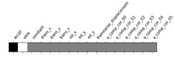
Fig 1: Plot of the contrast matrix

Then, the contrast matrix (Fig 1) was used to fit a first level General Linear Model (GLM). Finally, the nilearn.glm.compute_contrast method was used to compute the effect size and effect variance of the contrast of the model. Effect size represents the magnitude of difference between the view and recall runs. Effect variance represents the variance of the differences between the view and recall tasks. These results were saved as .nii files.

For each subject, the variance across all three runs was computed by using the compute_fixed_effects method. The three runs for each subject were combined into a single average run. Then, these results were used to compute the effect size and the effect variance between all 20 subjects, also known as random effects. Random effects looks at each voxel and runs a regression across subjects using the difference between each subject. These effect sizes and effect variances were stored into a folder and the original pre-processed fMRI data was deleted. This was done for storage purposes. Instead of having to store all 200 GBs of data at once, only storage of 87 MBs of data as contrasts was needed.

The design matrix was made using a column of ones of length 20, which is the number of subjects used in the dataset. Nilearn’s SecondLevelModel method was used to create the GLM for multiple subject fMRI data. Then, a second level GLM was fitted using the effect size for each subjects’ average run and the design matrix. Finally, a z-map was made using the second level GLM and multiple plots were created. These plots (shown in the results section) all used the same z-map and used various methods to set different thresholds for the z-map. These methods include uncorrected, false discovery rate correction, and Bonferroni correction.

Results

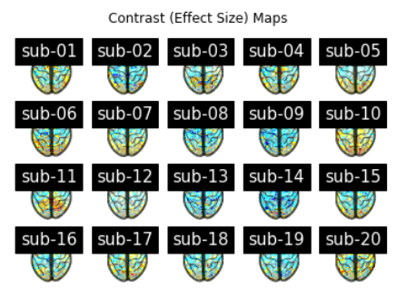
Fig 2: Effect Size contrasts of each subject

In Fig 2, the contrast maps (z-scores maps) corresponding to the effect size were plotted to visualize activation during viewing and recall tasks for each of the 20 subjects. There are similar general regions of activation between the 20 subjects.

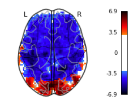
Fig 3: Plot cuts of a mask image using an uncorrected p < 0.001

First, a second level contrast (z-map) from the second level GLM was thresholded at an uncorrected p-value of 0.001 (p < 0.001) shown above in Fig 3. There is a 0.1% chance of returning an inactive voxel as active.

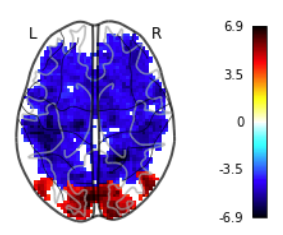
Fig 4: Plot cuts of a mask image using false discovery rate correction and set cluster threshold to 50 voxels

To remove some of the random data noise in the previous contrast, another second level contrast was created using a false discovery rate correction. Since a p-value of 0.001 was used, there is again a 0.1% chance of returning an inactive voxel as active. Clusters smaller than 50 voxels were removed, leading to greater confidence that the voxels identified as active are truly active. The plot is shown above in Fig 4.

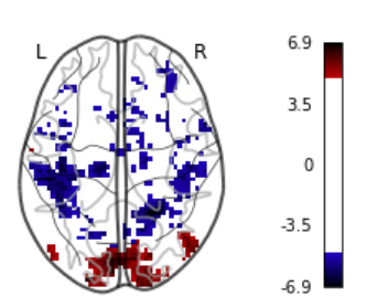
Fig 5: Plot cuts of a mask image using Bonferroni correction

Last, a second level contrast was performed using a strict Bonferroni correction in Fig 5 where the p-value is equal to (0.05) / (# of voxels in overall z-map) = (0.05) / (61 x 73 x 61) = 0.05 / 271633 = 1.841 * 10-7. This strict correction decreases the probability of obtaining false-positive results. There is a 1.841 * 10-5 probability of making any false detections.

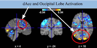
Fig 6: Interactive view of mask image slice using false discovery rate correction

Of the z-maps created for each of the 3 methods, the z-map created using false discovery rate correction was analyzed since it was the second most strict of the methods. An (x, y, z) position was chosen to look for significant regions of activation. The chosen position was (4, -24, 16). Voxel activity was found in the occipital lobe (Fig 6), which is the visual processing area of the brain. In addition, there is significant voxel activity in the Dorsal anterior cingulate cortex (dAcc), which is associated with “executive control, learning, adjustment, economic choice, and self-control” (Voloh et al., 2021).

Conclusion

In conclusion, different results from the original study were found. In Antony et al., 2020, the paper found neural activity in the ventral tegmental area (VTA), nucleus accumbens (NAcc), and prefrontal cortex. In this project, voxel activity in the occipital lobe and the Dorsal anterior cingulate cortex was observed. Significant voxel activity in the prefrontal cortex, VTA, or in the NAcc was not seen. This may be due to the paper using different thresholds for their plots. Another explanation could be that Antony et al., 2020 used a contrast other than effect size or effect variance.